
In 1985, Kasai, Namekawa, Koyana, and Omoto published a paper titled “Real-Time Two-Dimensional Blood Flow Imaging Using an Autocorrelation Technique” that changed the world of ultrasound imaging forever [1]. Considered impossible before, color flow mapping (CFM) has since become a must for every ultrasound system and is used routinely by sonographers.

This technique measures the projection of the blood flow velocity onto the ultrasound beam for a number of points in the image, and presents the estimates to the clinician using color coding (Fig. 1). The intensity is proportional to the brightness of the image, and the hue to the direction. Blue color indicates movement away from the transducer and red color towards the transducer.
The technique has been improved and refined over the years, but the basic principle has remained the same — the flow is estimated only along the ultrasound beam, and when the flow is perpendicular to the beam, it cannot be detected. The blood in the upper vessel shown in Fig. 1 flows from left to right, but due to geometry it looks as if it changes flow direction. Not only that, but clinicians must manually set the scan angle to correct for the angle dependence of the estimates. Furthermore, the estimates are increasingly unreliable at large angles. Today, the technique is used only for qualitative measurements.
In 1998, Jensen and Munk demonstrated a new estimation technique capable of estimating the full velocity vector independent of the angle [2–4], and in 2011, BK Medical (Herlev, Denmark) demonstrated the first commercial system based on the technique, thus opening a new page in the field of blood flow imaging. With a standard deviation of a mere 2 degrees of the estimates of flow angle (in any point in the image), this technique is paving the way from qualitative to quantitative blood flow measurements.
Measuring Blood Flow With Pulsed Ultrasound
Imagine standing beside a road and periodically take pictures. In the beginning, the road is empty. Then a car passes by from left to right. If the period between your pictures is sufficiently small, then the car will be present on a series of pictures — every time displaced a little to the right, relative to the previous picture.
The same principle is used in blood flow measurements using ultrasound. A series of pulses is sent along the same direction. Every time the pressure wave encounters an inhomogeneity, a signal is scattered back and recorded by the transducer. Blood is not homogeneous. Its main components are erythrocytes, leukocytes, platelets, plasma, and 0.9% saline. The erythrocytes, for example, give rise to Rayleigh scattering. The signal scattered back by the blood cells will vary from measurement to measurement in a manner similar to the experiment of taking photos of the street and passing cars.
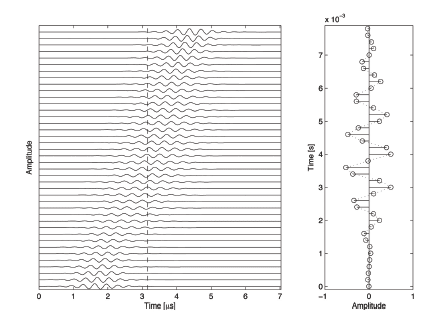
Figure 2 illustrates the measurement of blood flow. A single particle is moving away from the transducer. The reflected echo will therefore arrive every time a little bit later relative to the moment of sending a pulse. The vertical axis of the left plot corresponds to signals recorded from consecutive measurements in the same direction. The horizontal axis is time measured from pulse emission, which can be converted to scan depth after division by the speed of sound. If a single sample is taken from every measurement at a fixed time instance after pulse emission, a signal like the one on the right of Fig. 2 is formed. It oscillates. The oscillation frequency of this signal is popularly known as Doppler frequency, and is proportional to the speed with which the particle moves. This frequency can be estimated either by using a Fourier transform, or by estimating the phase shift as suggested by Kasai and coworkers.
Failing to Measure Velocity Vector
As shown in Fig. 2, the presence of Doppler frequency is caused by the presence of oscillations in the reflected signal. The figure only illustrates the signal along the ultrasound beam, but the ultrasound field is three-dimensional.
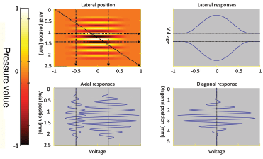
Figure 3 (top-left) illustrates the ultrasound field at a given time instance in the imaging plane (fixed value of the horizontal axis in Fig. 2). The signal reflected by moving scatterers and received by the transducer is given in the other three plots: scatterers moving perpendicular to the beam in the top-right plot; scatterers moving along the beam direction in the bottom-left plot; and diagonally moving scatterers in the bottom-right plot. The magnitude of the velocity is the same — only the direction and the spatial position of the scatterers are different. The fastest oscillations in the received signal are present when the scatterers move in the direction of the beam. There are no oscillations when the movement is perpendicular to the beam. The physics of the measurement situation makes it impossible to detect the lateral velocity using Doppler methods.
Transverse Oscillations
The full velocity vector is the sum of the axial (along the beam) and the transverse (perpendicular to the beam) velocity components. The question is how to find the transverse component.
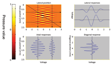
The idea introduced by Jensen and Munk is simple enough — if oscillations along beam direction make it possible to estimate the velocity component along the beam, then oscillations perpendicular to the beam direction will make it possible to estimate the transverse component. The principle is illustrated in Fig. 4.
It can be seen that all responses, from lateral, axial, and diagonal movements, contain oscillations. Thus a “transverse Doppler frequency” will be present, allowing the full velocity vector to be estimated using phase-estimation techniques.
Despite the simplicity of the idea, the creation of a double-oscillating ultrasound field is not obvious. In the initial work, Jensen and Munk use Fresnell approximation to design the beamforming parameters. Later, a pulsedplane wave field decomposition method was developed by Munk [2]. Various app roaches were tested — controlling the phase, the amplitude, or both of the received and/or transmitted signals.
Different approaches have been investigated over the years of how to find the lateral direction of the flow. The initial development has taken place at the Technical University of Denmark, led by professor Jørgen A. Jensen with the support of BK Medical ApS. Presently the vector flow imaging is implemented in the ultrasound systems of BK Medical ApS and awaits FDA approval.
Clinical Benefits
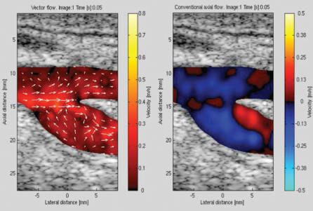
Some of the clinical benefits are obvious. For example, sonographers need less training to interpret the images, since the flow information includes both direction and magnitude as seen in Fig. 5, which shows the blood flow at the carotid bifurcation estimated using conventional blood flow estimation (right) and the newly developed vector flow imaging (left).
The presence of a vortex in the flow pattern of the CFM image is not obvious and requires an experienced user. The flow direction, on the other hand is indicated by the arrows in the vector flow image.
A less obvious benefit is the reduction of examination time. Vector Flow Imaging (VFI) is inherently angle-independent, and sonographers save time because they do not need to search for the best scan angle — unlike CFM (see Fig. 1), VFI has no blind angles.
Finally, the peak measured transverse velocity component is two times larger than the peak measured axial component for the same depth. This opens doors to new application areas where there is a need to measure fast blood flow parallel to the transducer surface, such as the flow in the fistulas of hemodialysis patients.

Because the method estimates both components — along the beam and perpendicular to the beam, it manifests higher overall precision than conventional CFM images. It has been used in a clinical study and compared to magnetic resonance contrast angiography (MRA) by calculating the stroke volume. The correlation between the stroke volumes is estimated using VFI, and MRA is above 91%. The authors concluded that VFI can be used for reliable quantitative flow estimation and have even raised the question of whether or not VFI should replace MRA as the gold standard for flow estimation.
What’s Next?
Looking at the research papers published at the annual IEEE International Ultrasonics Symposium, there is no doubt that vector flow imaging techniques represent the future of ultrasound blood flow measurements. An increasing number of papers focus on high frame rate imaging.
Research conducted at the Technical University of Denmark in collaboration with the Royal Hospital in Copenhagen and BK Medical ApS shows that combining high-frame rate acquisition with vector flow estimation reveals new patterns of blood flow not visible with other techniques [6].
An example is shown in Fig. 6. One can see that the blood flows in a circular manner along the vessel wall. What these disturbances in these flow patterns may indicate about the health of the patient are yet to be determined by clinical research. One thing, however, is clear: 1D qualitative blood flow imaging will soon be replaced by 2D and even 3D quantitative vector flow imaging.
This article was written by Svetoslav Ivanov Nikolov, System Engineer for BK Medical ApS, Herlev, Denmark. For more information, Click Here .
References
- C. Kasai, K. Namekawa, A. Koyano, and R. Omoto, “Real-Time Two-Dimensional Blood Flow Imaging Using an Autocorrelation Technique,” IEEE Trans. Son. Ultrason., vol. 32, no. 3, pp. 458-464, 1985.
- P. Munk, “Estimation of blood velocity vectors using ultrasound,” Department of Information Technology, Technical University of Denmark, 2000.
- J. A. Jensen and P. Munk, “A new method for estimation of velocity vectors.,” IEEE transactions on ultrasonics, ferroelectrics, and frequency control, vol. 45, no. 3, pp. 837-51, Jan. 1998.
- J. A. Jensen, “A new estimator for vector velocity estimation,” IEEE Trans. Ultrason., Ferroelec., Freq. Contr., vol. 48, no. 4, pp. 886-894, 2001.
- K. L. Hansen et al., “In vivo comparison of three ultrasound vector velocity techniques to MR phase contrast angiography.,” Ultrasonics, vol. 49, no. 8, pp. 659-67, Dec. 2009.
- K. L. Hansen et al., “In vivo comparison of three ultrasound vector velocity techniques to MR phase contrast angiography.,” Ultrasonics, vol. 49, no. 8, pp. 659-67, Dec. 2009.